Safety in numbers. Part 4

In the last 3 parts, we have covered just 2 basic types about failures that can be encountered in any flight. Now, that’s those that effect single systems, and their subsystems and those that impact a whole aircraft as a common effect.

The single failure cases were considered assuming that failures were independent. That is something fails but the effects are contained within one system.

There’s a whole range of other failures where dependencies exist between different systems as they fail. We did mention the relationship between a fuel system and a propulsion system. Their coexistence is obvious. What we need to do is to go beyond the obvious and look for relationships that can be characterised and studied.

At the top of my list is a condition where a cascade of failures ripple through aviation systems. This is when a trigger event starts a set of interconnected responses. Videos of falling dominoes pepper social media and there’s something satisfying about watching them fall one by one.

Aircraft systems cascade failures can start with a relatively minor event. When one failure has the potential to precipitate another it’s important to understand the nature of the dependency that can be hardwired into systems, procedures, or training.

It’s as well to note that a cascade, or avalanche breakdown may not be straightforward as it is with a line of carefully arranged dominos. The classical linear way of representing causal chains is useful. The limitation is that dominant, or hidden interdependencies can exist with multiple potential paths and different sequences of activation.

The next category of failure is a variation on the common-mode theme. This has more to do with the physical positions of systems and equipment on an aircraft. For example, a localised fire, flood, or explosion can defeat built-in redundancies or hardened components.

Earlier we mentioned particular risks. Now, we need to add to the list; bird strike, rotor burst, tyre burst and battery fires. The physical segregation of sub-systems can help address this problem.

Yes, probabilistic methods can be used to calculate likelihood of these failure conditions occurring.

The next category of failure is more a feature of failure rather than a type of failure. Everything we have talked about, so far, may be evident at the moment of occurrence. There can then be opportunities to take mitigating actions to overcome the impact of failure.

What about those aircraft systems failures that are dormant? That is that they remain passive and undetected until a moment when systems activation is needed or there’s demand for a back-up. One example could be just that, an emergency back-up battery that has discharged. It’s then unavailable when it’s needed the most. Design strategies like, pre-flight checks, built-in-test and continuous monitoring can overcome some of these conditions.

Safety in numbers, Part 3

The wind blows, the sun shines, a storm brews, and rain falls. Weather is the ultimate everyday talking point. Stand at a bus stop, start a conversation and it’ll likely be about the weather. Snow, sleet, ice or hail the atmosphere can be hostile to our best laid plans. It’s important to us because it affects us all. It has a common effect.

We started a discussion of common-mode failures in earlier paragraphs. We’ll follow it up here. Aircraft systems employ an array of strategies to address combinations and permutations of failure conditions. That said, we should not forget that these can be swamped by common-mode effects.

Environmental effects are at the top of the list of effects to consider. It’s a basic part of flying that the atmosphere changes with altitude. So, aircraft systems and equipment that work well on the ground may have vulnerabilities when exposed to large variations in temperatures, atmospheric pressure, and humidity.

Then there’s a series of effects that are inherent with rotating machinery and moving components. Vibration, shock impacts and heat all need to be addressed in design and testing.

It is possible to apply statistical methods to calculate levels of typical exposure to environmental effects, but it is more often the case that conservative limits are set as design targets.

Then there are particular risks. These are threats that, maybe don’t happen everyday but have the potential to be destructive and overcome design safety strategies. Electromagnetic interference and atmospheric disturbances, like lightning and electrostatic discharge can be dramatic. The defences against these phenomena can be to protect systems and limit impacts. Additionally, the separation or segregation of parts of systems can take advantage of any built-in redundancies.

Some common-mode effects can occur due to operational failures. The classic case is that of running out of fuel or electrical power. This is where there’s a role for dedicated back-up systems. It could be a hydraulic accumulator, a back-up battery, or a drop-out ram air turbine, for example.

Some common-mode effects are reversable and tolerable in that they don’t destroy systems and equipment but do produce forms of performance degradation. We get into the habit of talking about failure as if they are absolute, almost digital, but it’s an analogue world. There’s a range of cases where adjustments to operations can mitigate effects on aircraft performance. In fact, an aircraft’s operational envelope can be adjusted to ensure that it remains in a zone where safe flight and landing are possible, however much systems are degraded.

Probabilities can play a role in such considerations. Getting reliable data on which to base sound conclusions is often the biggest challenge. Focusing on maintaining a controllable aircraft with a minimum of propulsion, in the face of multiple hazards takes a lot of clear thought.

Safety in numbers. Part 1

It’s a common misconception that the more you have of something the better it is. Well, I say, misconception but in simple cases it’s not a misconception. For safety’s sake, it’s common to have more than one of something. In a classic everyday aircraft that might be two engines, two flight controls, two electrical generators and two pilots, so on.

It seems the most common-sense of common-sense conclusions. That if one thing fails or doesn’t do what it should we have another one to replace it. It’s not always the case that both things work together, all the time, and when one goes the other does the whole job. That’s because, like two aircraft engines, the normal situation is both working together in parallel. There are other situations where a system can be carrying the full load and another one is sitting there keeping an eye on what’s happening ready to take over, if needed.

This week, as with many weeks, thinkers and politicians have been saying we need more people with a STEM education (Science, Technology, Engineering, and Math). Often this seems common-sense and little questioned. However, it’s not always clear that people mean the same things when talking about STEM. Most particularly it’s not always clear what they consider to be Math.

To misquote the famous author H. G. Wells: Statistical thinking may, one day be as necessary as the ability to read and write. His full quote was a bit more impenetrable, but the overall meaning is captured in my shorten version.

To understand how a combination of things work together, or not, some statistical thinking is certainly needed. Fighting against the reaction that maths associated with probabilities can scare people off. Ways to keep our reasoning simple do help.

The sums for dual aircraft systems are not so difficult. That is provided we know that the something we are talking about is reliable in the first place. If it’s not reliable then the story is a different one. For the sake of argument, and considering practical reality let say that the thing we are talking about only fails once every 1000 hours.

What’s that in human terms? It’s a lot less than a year’s worth of daylight hours. That being roughly half of 24 hours x 7 days x 52 weeks = 4368 hours (putting aside location and leap years). In a year, in good health, our bodies operate continuously for that time. For the engineered systems under discussion that may not be the case. We switch the on, and we switch them off, possibly many times in a year.

That’s why we need to consider the amount of time something is exposed to the possibility of failure. We can now use the word “probability” instead of possibility. Chance and likelihood work too. When numerically expressed, probabilities range from 0 to 1. That is zero being when something will never happen and one being when something will always happen.

So, let’s think about any one hour of operation of an engineered system, and use the reliability number from our simple argument. We can liken that, making an assumption, to a probability number of P = 1/1000 or 1 x 10⁻³ per hour. That gives us a round number that represents the likelihood of failure in any one hour of operation of one system.

Now, back to the start. We have two systems. Maybe two engines. That is two systems that can work independently of each other. It’s true that there are some cases where they may not work independently of each other but let’s park those cases for the moment.

As soon as we have more than one thing we need to talk of combinations. Here the simple question is how many combinations exist for two working systems?

Let’s give them the names A and B. In our simplified world either A or B can work, or not work when needed to work. That’s failed or not failed, said another way. There are normally four combinations that can exist. Displayed in a table this looks like:

A okB ok
A failsB ok
A okB fails
A failsB fails
Table 1

This is all binary. We are not considering any near failure, or other anomalous behaviour that can happen in the real world. We are not considering any operator intervention that switches on or switches off our system. We are looking at the probability of a failure happening in a period of operation of both systems together.

Now, let’s say that the systems A and B each have a known probability of failure.

Thus, the last line of the table becomes: P4 = PA and PB

That is in any given hour of operation the chances of both A and B failing together are the product of their probabilities. Assuming the failures to be random.

Calculating the last line of the table becomes: P4 = PA x PB

In the first line of the table, we have the case of perfection. Simultaneous operation is not interrupted, even though we know both A and B have a likelihood of failure in any one hour of operation.

Thus, the first line becomes: P1 = (1 – PA) x (1 – PB)

Which nicely approximates to P1 = 1, given that 1/1000 is tiny by comparison.

The cases where either A or B fails are in the middle of the table.

P2 = PA x (1 – PB) together with P3 = (1 – PA) x PB

Thus, using the same logic as above the probability of A or B failing is PA + PB

It gets even better if we consider the two systems to be identical. Namely, that probabilities PA and PB  are equal.

A double failure occurs at probability P2

A single failure occurs at probability 2P

So, two systems operating in parallel there’s a decreased the likelihood of a double failure but an increase in the likelihood of a single failure. This can be taken beyond an arrangement with two systems. For an arrangement with four systems, there’s a massively decreased likelihood of a total failure but four times the increase in the likelihood of a single failure. Hence my remark at the beginning. 

[Please let me know if this is in error or there’s a better way of saying it]